Column-Major Order: Storing a Grid Column by Column

Column-Major Order: Storing a Grid Column by Column

Computer memory is one long, straight line of boxes. But a 2D array (a grid with rows and columns) is not a straight line — it has shape. So before the computer can store a grid in memory, it has to "flatten" it into a single line. There are two common ways to do this. One is row-major order (store one full row at a time). The other — the one we learn here — is column-major order.

In column-major order, the rule is simple: the elements that sit in the same column go next to each other in memory. You pour the grid into memory one column at a time, top to bottom, then move to the next column.

A concrete example

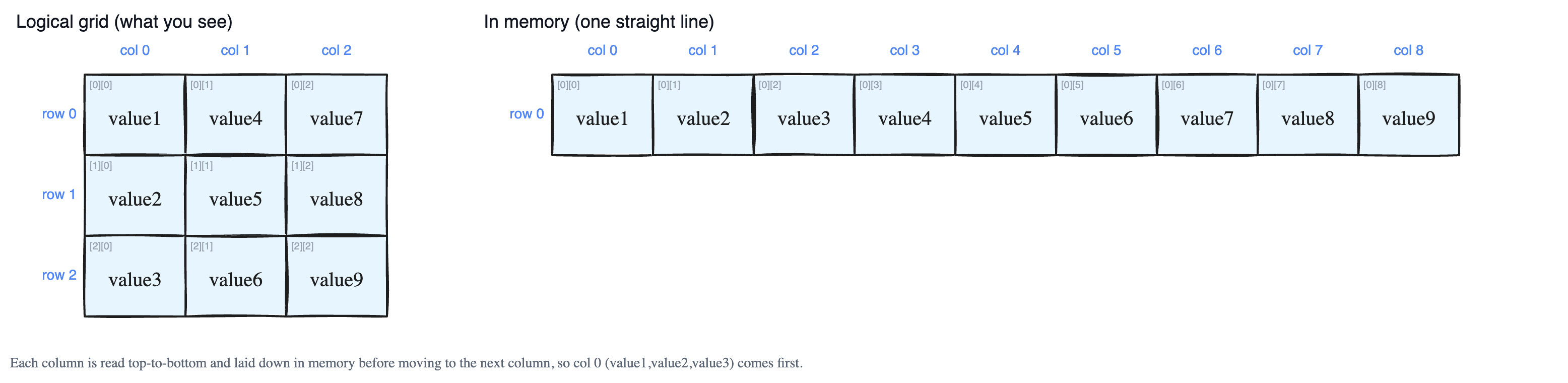
Take this 3×3 grid:

value1  value4  value7
value2  value5  value8
value3  value6  value9

Read it column by column, going down each column first:

• First column (top to bottom): value1, value2, value3
• Second column: value4, value5, value6
• Third column: value7, value8, value9

So in memory the line looks like this:

value1 value2 value3 value4 value5 value6 value7 value8 value9

Notice value1, value2, value3 are neighbors — they were the first column. This is the opposite of row-major order, which would have stored value1, value4, value7 together (the first row). That is why column-major order is often called the transpose (the flipped version) of row-major order.

"The highest dimension moves fastest"

Here is the key idea, stated in plain words. Think of a 2D array as array[row][column]. To walk through every cell in column-major order, you change the row index (the leftmost, "highest" dimension) as fast as you can, and only after a whole column is done do you bump up the column index.

In other words, the first index changes most often:

[0][0]  ->  [1][0]  ->  [2][0]   (finish column 0)
[0][1]  ->  [1][1]  ->  [2][1]   (then column 1)
[0][2]  ->  [1][2]  ->  [2][2]   (then column 2)

The book shows this happening one element at a time: it places the value at [0][0] into memory, then [1][0], then [2][0], and keeps going. This same idea scales up to arrays with many dimensions: you always move the highest (leftmost) dimension the fastest and the lowest dimension the slowest, mapping every value into the memory line until all the data is stored.

Which languages use it?

Most everyday languages (like C, C++, Java) use row-major order. Column-major order is the choice of math and science languages such as Fortran, MATLAB, and Julia. If you ever mix code from these worlds, knowing which order is used helps you avoid mixing up rows and columns.

Finding an element's address with a formula

Once you know the layout rule, you can jump straight to any element's address in memory without scanning — just compute it. You need three things:

1. The base address — where the array starts in memory (in the book's picture this is 2).
2. The size of the base type — how many bytes one element takes.
3. The sizes of each dimension, written Dn x Dn-1 x ... x D1.

For an element at index In, In-1, ... I1, the address is:

address = base address
        + size of base type * ( In
                              + Dn * ( In-1
                              + Dn-1 * ( In-2
                              + ... + D2 * I1 ) ... ) )

Read it from the inside out. The innermost index is multiplied and added step by step, each time scaled by the size of a dimension. Because the first index In has no multiplier, it moves one step at a time in memory — which matches the rule "the highest dimension moves fastest." The size of the very last dimension never appears in the formula, exactly like how, in row-major order, the size of the first dimension is never needed.

The takeaway

Column-major order flattens a multidimensional array by walking down columns first, keeping each column's elements together in memory. The leftmost index changes fastest, and a single address formula lets you find any element instantly.